The sequence of sets S(0), S(1), S(2), S(3), .... that are constructed this way form a Cauchy sequence in the Hausdorff metric, and \(\displaystyle S = \lim_{n \rightarrow \infty} S(n)\) is the Koch snowflake [Proof].
Iteration
Click the iterations to the left for another illustration of how the snowflake is formed.

IFS
Animation
(hexagons)
IFS
Demonstration
Video
|
\({f_1}({\bf{x}}) = \left[ {\begin{array}{*{20}{c}}
{ 1/2} & {- \sqrt 3 /6 } \\
{\sqrt 3 /6} & { 1/2} \\
\end{array}} \right]{\bf{x}} \) |
scale by \(1/ \sqrt{3} \), rotate by 30° |
|
\({f_2}({\bf{x}}) = \left[ {\begin{array}{*{20}{c}}
{ 1/3} & {0} \\
{ 0} & { 1/3} \\
\end{array}} \right]{\bf{x}} + \left[ {\begin{array}{*{20}{c}}
{1/\sqrt 3 } \\
{1/3} \\
\end{array}} \right]\) |
scale by 1/3 |
|
\({f_3}({\bf{x}}) = \left[ {\begin{array}{*{20}{c}}
{ 1/3} & {0} \\
{ 0} & { 1/3} \\
\end{array}} \right]{\bf{x}} + \left[ {\begin{array}{*{20}{c}}
{0} \\
{2/3} \\
\end{array}} \right]\) |
scale by 1/3 |
|
\({f_4}({\bf{x}}) = \left[ {\begin{array}{*{20}{c}}
{ 1/3} & {0} \\
{0} & { 1/3} \\
\end{array}} \right]{\bf{x}} + \left[ {\begin{array}{*{20}{c}}
{-1/ \sqrt 3} \\
{1/3} \\
\end{array}} \right]\) |
scale by 1/3 |
|
\({f_5}({\bf{x}}) = \left[ {\begin{array}{*{20}{c}}
{ 1/3} & {0} \\
{ 0} & { 1/3} \\
\end{array}} \right]{\bf{x}} + \left[ {\begin{array}{*{20}{c}}
{- 1/\sqrt 3} \\
{- 1/3} \\
\end{array}} \right]\) |
scale by 1/3 |
|
\({f_6}({\bf{x}}) = \left[ {\begin{array}{*{20}{c}}
{ 1/3} & {0} \\
{ 0} & { 1/3} \\
\end{array}} \right]{\bf{x}} + \left[ {\begin{array}{*{20}{c}}
{0} \\
{- 2/3} \\
\end{array}} \right]\) |
scale by 1/3 |
|
\({f_7}({\bf{x}}) = \left[ {\begin{array}{*{20}{c}}
{ 1/3} & {0} \\
{ 0} & { 1/3} \\
\end{array}} \right]{\bf{x}} + \left[ {\begin{array}{*{20}{c}}
{1/ \sqrt 3} \\
{- 1/3} \\
\end{array}} \right]\) |
scale by 1/3 |
Koch converging
to his snowflake!
IFS
Animation
(line segments)
IFS
Animation
(triangles)
|
\({f_1}({\bf{x}}) = \left[ {\begin{array}{*{20}{c}}
{ - 1/6} & {\sqrt 3 /6} \\
{ - \sqrt 3 /6} & { - 1/6} \\
\end{array}} \right]{\bf{x}} + \left[ {\begin{array}{*{20}{c}}
{1/6} \\
{\sqrt 3 /6} \\
\end{array}} \right]\) |
scale by 1/3, rotate by −120° |
|
\({f_2}({\bf{x}}) = \left[ {\begin{array}{*{20}{c}}
{ 1/6} & {- \sqrt 3 /6} \\
{ \sqrt 3 /6} & { 1/6} \\
\end{array}} \right]{\bf{x}} + \left[ {\begin{array}{*{20}{c}}
{1/6} \\
{\sqrt 3 /6} \\
\end{array}} \right]\) |
scale by 1/3, rotate by 60° |
|
\({f_3}({\bf{x}}) = \left[ {\begin{array}{*{20}{c}}
{ 1/3} & {0} \\
{ 0} & { 1/3} \\
\end{array}} \right]{\bf{x}} + \left[ {\begin{array}{*{20}{c}}
{1/3} \\
{\sqrt 3 /3} \\
\end{array}} \right]\) |
scale by 1/3 |
|
\({f_4}({\bf{x}}) = \left[ {\begin{array}{*{20}{c}}
{ 1/6} & { \sqrt 3 /6} \\
{- \sqrt 3 /6} & { 1/6} \\
\end{array}} \right]{\bf{x}} + \left[ {\begin{array}{*{20}{c}}
{2/3} \\
{\sqrt 3 /3} \\
\end{array}} \right]\) |
scale by 1/3, rotate by −60° |
|
\({f_5}({\bf{x}}) = \left[ {\begin{array}{*{20}{c}}
{ 1/2} & {- \sqrt 3 /6} \\
{ \sqrt 3 /6} & { 1/2} \\
\end{array}} \right]{\bf{x}} + \left[ {\begin{array}{*{20}{c}}
{1/3} \\
{0} \\
\end{array}} \right]\) |
scale by \(1/\sqrt{3} \), rotate by 30° |
|
\({f_6}({\bf{x}}) = \left[ {\begin{array}{*{20}{c}}
{ -1/3} & {0} \\
{ 0} & { -1/3} \\
\end{array}} \right]{\bf{x}} + \left[ {\begin{array}{*{20}{c}}
{2/3} \\
{0} \\
\end{array}} \right]\) |
scale by 1/3, rotate by 180° |
|
\({f_7}({\bf{x}}) = \left[ {\begin{array}{*{20}{c}}
{ 1/3} & {0} \\
{ 0} & { 1/3} \\
\end{array}} \right]{\bf{x}} + \left[ {\begin{array}{*{20}{c}}
{2/3} \\
{0} \\
\end{array}} \right]\) |
scale by 1/3 |
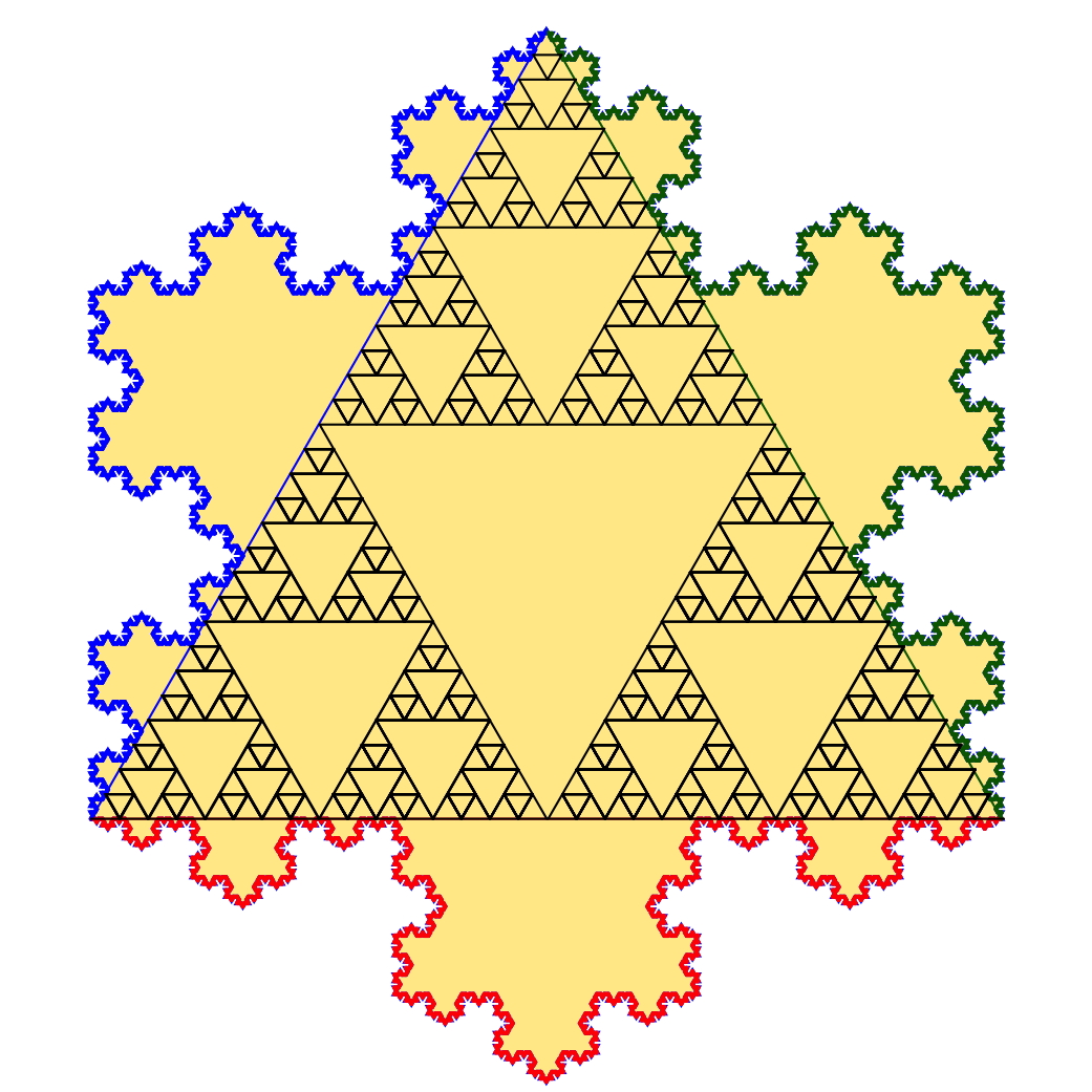
[Click for Snowflake with the Sierpinski Triangle]
This boundary can be constructed by the following L-system:
Angle 60
Axiom F++F++F
F —> F−F++F−F
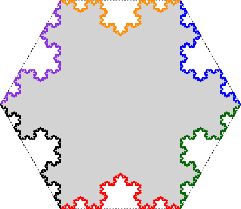
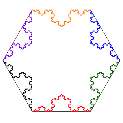
The boundary of the snowflake can also be considered to consist of six copies of the Koch curve placed around the six sides of a regular hexagon and facing inwards.
This boundary can be constructed by the following L-system:
Angle 60
Axiom F+F+F+F+F+F
F —> F+F−−F+F
The six copies of the Koch curve around a hexagon consists of three pairs, each of which form a Koch curve around an equilateral triangle inscribed in the hexagon. Toggle between the two versions using the buttons below.
\[1 = 6{\left( {\frac{1}{3}} \right)^d} + {\left( {\frac{1}{{\sqrt 3 }}} \right)^d}\]
The unique solution to this equation is d = 2. Notice, however, that the boundary of the Koch snowflake consists of multiple copies of the Koch curve, which has a fractal dimension of 1.26186.
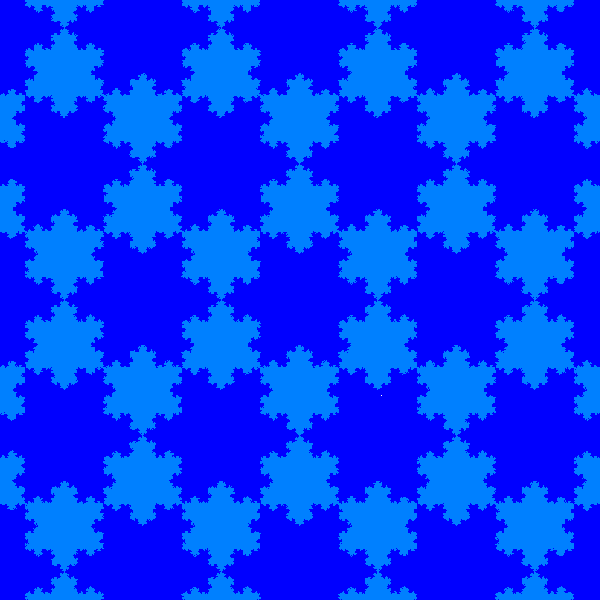
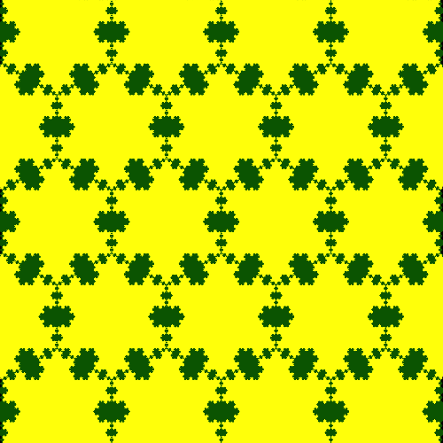
The Koch snowflake along with copies scaled by \(1/\sqrt 3\) and rotated by 30° can be used to tile the plane [Example 1, Example 2], or copies of the Koch snowflake and anti-snowflake can also tile the plane [Example]. See details.
The length of the boundary of S(n) at the nth iteration of the construction is \(3{\left( {\frac{4}{3}} \right)^n} s\), where s denotes the length of each side of the original equilateral triangle. Therefore the Koch snowflake has a perimeter of infinite length.
The area of S(n) is \[\frac{{\sqrt 3 {s^2}}}{4}\left( {1 + \sum\limits_{k = 1}^n {\frac{{3 \cdot {4^{k - 1}}}}{{{9^k}}}} } \right).\] Letting n go to infinity shows that the area of the Koch snowflake is \(\dfrac{2\sqrt 3}{5}{s^2}\) . Since the area of the original equilateral triangle is \(\dfrac{\sqrt 3}{4}{s^2}\), this means that the area of the snowflake is 8/5 times the area of the original equilateral triangle. It is also possible to compute the area of the snowflake using fractal similarity. [Details]
Notice in particular that the snowflake has a finite area bounded by a perimeter of infinite length! This apparent paradox plays a role in the novel The Curve of the Snowflake by William Grey Walter.
Start with an equilateral triangle T as before. Place three copies of a Koch curve around the three edges of T but pointed inside T. This creates the Koch anti-snowflake as shown above on the left. The region bounded by this curve is also known as the Koch anti-snowflake. As a slightly different variation, rather than adding 3 scaled copies of the triangle T to the outside, point the new triangles into the interior of T and remove those regions from T. This leaves three diamond shaped regions, each of which consists of two scaled copies of T, for a total of 6 new equilateral triangles. Now repeat the construction on each of those 6 triangles, and so on. This produces the figure on the right above. The outside boundary of this figure is the curve shown on the left. Click on the link above for more details. (The name "anti-snowflake curve" also appears in the 1940 book Mathematics and Imagination by Kasner and Newman referenced above.)
Animation
This variation on the Koch snowflake was created by William Gosper. Start with a pattern of seven regular hexagons. Eight vertices are connected as shown above to create the basic red motif. The red line segments are oriented by the arrows. Now replace each red line segment by a copy of the motif scaled by \(1/ \sqrt 7 \) such that the copy lies to the left of the oriented edge it is replacing. Notice that this will place the copy of the motif inside the hexagon containing that edge. This recursive procedure is continued and in the limit will produce the image of a space filling curve shown above, known as the flowsnake (a play on words of snowflake). This version of Gosper's flowsnake was first described by Martin Gardner in one of this Mathematical Games columns in Scientific American. Click on the link above for more details.
This variation is from the book Curious Curves by Darst, Palagallo, and Price. The three scaled copies of the initial equilateral triangle are taken from the interior of the equilateral triangle after it has been subdivided into 9 equal parts. This recursive procedure is continued and the limit will produce the image of a snowflake. It is shown in the book that the snowflake is actually a curve, that is, the image of a nontrivial continuous map from [0,1] into the plane.