Start with a solid (filled) equilateral triangle S(0). Divide this into four smaller equilateral triangles using the midpoints of the three sides of the original triangle as the new vertices. Remove the interior of the middle triangle (that is, do not remove the boundary) to get S(1). Now repeat this procedure on each of the three remaining solid equilateral triangles to obtain S(2).
Continue to repeat the construction to obtain a decreasing sequence of sets
$$ S(0) \supset S(1) \supset S(2) \supset S(3) \supset \cdots $$
The Sierpinski gasket, also known as the Sierpinski triangle, is the intersection of all the sets in this sequence, that is, the set of points that remain after this construction is repeated infinitely often.
The set S(1) can also be obtained by scaling three copies of S(0) each by a factor of r=1/2 and then translating two of the smaller triangles to form the desired arrangement. If we imagine the bottom side of S(0) to lie along the x-axis with the vertices at the origin and at the point (1,0), then two of the scaled triangles would have to be translated so that the lower left vertices are at (1/2, 0) and \((1/4, \sqrt 3 /4)\) respectively. This yields the following iterated function system.
|
\({f_1}({\bf{x}}) = \left[ {\begin{array}{*{20}{c}}
{1/2} & 0 \\
0 & {1/2} \\
\end{array}} \right]{\bf{x}}\) |
scale by r |
|
\({f_2}({\bf{x}}) = \left[ {\begin{array}{*{20}{c}}
{1/2} & 0 \\
0 & {1/2} \\
\end{array}} \right]{\bf{x}} + \left[ {\begin{array}{*{20}{c}}
{1/2} \\
0 \\
\end{array}} \right]\) |
scale by r |
| \({f_3}({\bf{x}}) = \left[ {\begin{array}{*{20}{c}} {1/2} & 0 \\ 0 & {1/2} \\ \end{array}} \right]{\bf{x}} + \left[ {\begin{array}{*{20}{c}} {1/4} \\ {\sqrt{3}/4} \\ \end{array}} \right]\) | scale by r |
IFS
Animation
3 different
initial sets
IFS
Animation
Sierpinski
converges to
his own triangle!
IFS
Animation
Circumscribed
Circles
If you apply the IFS to S(1), you will get S(2). Apply it to S(2) to get S(3), and continue to do this indefinitely. The Sierpinski gasket is the attractor for this IFS. This means that if you apply the iterated function system repeatedly beginning with any initial compact set (such as S(0)), then the resulting images will converge to the Sierpinski gasket, and applying the IFS to the Sierpinski gasket itself will just reproduce the same image. To see some examples of this behavior, view the IFS animation with three different initial sets. You can even make Sierpinski himself converge to his own gasket!
Because of the rotational symmetry of an equilateral triangle, there is second iterated function system that has the Sierpinski gasket as its attractor. In addition to scaling by a factor of r=1/2, rotate two of the triangles by 120° and -120°, then translate.
This yields the IFS given by
|
\({f_1}({\bf{x}}) = \left[ {\begin{array}{*{20}{c}}
{ - 1/4} & {\sqrt{3}/4} \\
{ - \sqrt{3}/4} & { - 1/4} \\
\end{array}} \right]{\bf{x}} + \left[ {\begin{array}{*{20}{c}}
{1/4} \\
{\sqrt{3}/4} \\
\end{array}} \right]\) |
scale by r, rotate by −120° |
|
\({f_2}({\bf{x}}) = \left[ {\begin{array}{*{20}{c}}
{ 1/2} & {0} \\
{ 0} & { 1/2} \\
\end{array}} \right]{\bf{x}} + \left[ {\begin{array}{*{20}{c}}
{1/4} \\
{\sqrt{3}/4} \\
\end{array}} \right]\) |
scale by r |
| \({f_3}({\bf{x}}) = \left[ {\begin{array}{*{20}{c}} { - 1/4} & {- \sqrt{3}/4} \\ { \sqrt{3}/4} & { - 1/4} \\ \end{array}} \right]{\bf{x}} + \left[ {\begin{array}{*{20}{c}} {1} \\ {0} \\ \end{array}} \right]\) | scale by r, rotate by 120° |
IFS
Animation
via Line
Segments
If the iterated function system given above is applied to an initial set that is a horizontal line segment, then the first three iterations would be the following:

The construction can also be described this way. Begin with a horizontal line segment. As the first iteration, replace this segment with three segments, each scaled by 1/2, in such a way that the original segment would be the base of a trapezoid with the top parallel to the base. Call this trapezoid (minus the base) the motif. For the second iteration, replace each of the line segments in the first iteration with a copy of the motif scaled by (1/2)2, using the following replacement rules for how to place the copies of the scaled motif relative to the segments in the previous iteration.
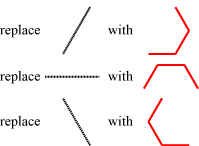
Continue this replacement for each new iteration. At the nth iteration, replace each of the segments of the previous iteration with copies of the motif scaled by a ratio of (1/2)n using the replacement rules shown above. The limit of the iterations as n goes to infinity will be the Sierpinski gasket. Watch the animation to see this convergence.
Zoom
Animation
L-System
Animation ver 1
Suppose we started with just the axiom F, that is, just one side of the triangle. The first iteration generated by the rule given above would be the following
We can see how the rule generates the boundary of the removed inside triangle. Repeated iterations will form more of the interior triangles but will leave out the other two sides of the main triangle. If you watch L-system animation version 1, you will notice that the animation seems to pause occasionally. This is because this L-system will trace some of the sides of the triangles more than once. To see how this happens, watch L-system animation version 2.
L-System
Animation ver 3
Angle 60
Axiom FX
F —> Z
X —> +FY-FX-FY+
Y —> -FX+FY+FX-
This a bit different in that each curve never intersects with itself as with the first L-system. As such, this construction illustrates that the Sierpinski gasket is actually a plane curve. It corresponds to the construction illustrated above with the second of the iterated function systems when the initial set is a horizontal line.
Below is the fourth iteration of each L-system. Watch the animations for a more detailed view.


$$\sum\limits_{k = 1}^3 {{r^d}} = 1\quad \Rightarrow \quad d = \frac{{\log (1/3)}}{{\log (r)}} = \frac{{\log (1/3)}}{{\log (1/2)}} = \frac{{\log (3)}}{{\log (2)}} = 1.58496$$
The following figure shows six Sierpinski gaskets put together in a hexagonal shape. This "curve" also has some interesting topological properties that Sierpinski discussed in his 1915 and 1916 papers. Also see reference [3].
We remove "all" of the area of the initial triangle in constructing the Sierpinski gasket. But of course there are many points still left in the gasket.
What is the average distance between two points in a unit Sierpinski gasket? The answer is 466 / 885 = 0.52655. Ian Stewart [17] credits this result to Andreas Hinz and describes how the use of graph theory to analyze the n-disk Tower of Hanoi puzzle can be used to calculate this average distance.
An interesting connection also exists between Pascal's Triangle and the Sierpinski Gasket. There's even some applications to electric circuits!
Could the Sierpinski gasket have captured the imagination of neolithic people in Ireland 5000 years ago? Look at these images and decide for yourself. An article by Elisa Conversano and Laura Tedeschini-Lalli in the 2011 Journal of Applied Mathematics illustrates designs from 11th century Rome churches that are similar to Sierpinski gaskets. Snow artist Simon Beck created a Sierpinski triangle pattern in snow with snowshoes. This was also the February image for the 2013 Calendar of Mathematical Imagery from the American Mathematical Society. Mathematician and artist David A. Reimann created Binomial Pursuit which depicts a Sierpinski triangle where a pursuit triangle is used on the interior triangles, and a simple black outlined triangle is used on the exterior triangles. It was featured as the cover art for the June 2016 issue of Mathematics Magazine.
Tom Edgar's YouTube channel on Mathematical Visual Proofs includes animations of Six Sierpinski Triangle Constructions.
The pedal triangle of an acute triangle T is the triangle formed by the three points that lie at the feet of the three altitudes of T, i.e. from each vertex drop a perpendicular to the opposite side until it intersects with that side. The pedal triangle divides the original triangle into four smaller triangles. Remove the interior of the pedal triangle, then repeat the construction on the remaining three triangles.
The Sierpinski gasket is formed by scaling an equilateral triangle by the factor r= 1/2. Instead of using this scaling factor, however, we can scale the equilateral triangle by a number λ between 0 and 1, make three copies, then translate them to fit back within the original triangle.
Allow the top triangle to rotate around its center. Each rotation produces a different iterated function system with a different attractor. Click on the link above to see an animation of how that changes the Sierpinski gasket.
The Sierpinski gasket can also be constructed by starting with a square that is subdivided into four equal subsquares, then removing the upper right subsquare. By performing one of the 8 symmetry transformations of a square on each of the three remaining subsquares during each step of the iteration, many variations of the Sierpinski gasket can be obtained. Click on the link above for more details and examples of such fractals (such as the one below).
Perform the usual construction for the Sierpinski gasket, but rather than remove the middle triangle, remove the top triangle. The remaining three triangles may be rotated by 120° or 240°, or reflected across one of the altitudes, to form variations on the Sierpinski gasket. Click on the link above for more details and examples of such fractals (such as the one below).
The example of a triangle fractal shown above shows a sequence of Sierpinski triangles shrinking in size. A different version of this is illustrated in the book Brainfilling Curves, by Jeffrey Ventrella. He constructs this as family of non-crossing curves in what he describes as a root4 triangle grid family. It is also the attractor of an IFS with three functions that mimic the usual construction of a Sierpinski triangle. Click on the button to the left for a demonstration.
|
\({f_1}({\bf{x}}) = \left[ {\begin{array}{*{20}{c}}
{ 1/4} & {\sqrt{3}/4} \\
{ \sqrt{3}/4} & { - 1/4} \\
\end{array}} \right]{\bf{x}}\) |
|
\({f_2}({\bf{x}}) = \left[ {\begin{array}{*{20}{c}}
{ - 1/4} & {- \sqrt{3}/4} \\
{ \sqrt{3}/4} & { - 1/4} \\
\end{array}} \right]{\bf{x}} + \left[ {\begin{array}{*{20}{c}}
{1/2} \\
{0} \\
\end{array}} \right]\) |
| \({f_3}({\bf{x}}) = \left[ {\begin{array}{*{20}{c}} { 1/2} & {0} \\ { 0} & { 1/2} \\ \end{array}} \right]{\bf{x}} + \left[ {\begin{array}{*{20}{c}} {1/2} \\ {0} \\ \end{array}} \right]\) |
This iterated function system produces the following fractal which actually has six-fold rotational symmetry (in addition to several reflective symmetries). This is because the fixed attractor is a filled-in hexagon [Details]. It is colored using pixel counting (the color depends on how many times a particular pixel is plotted during the drawing of the fractal using the random chaos game algorithm). More details on symmetric fractals can be found here and in the book by Field and Golubitsky.


See a similar image implemented in Desmos by Eric Berger.
