Construction
Animation
Recall that \({\bf{r}} = \frac{1}{{\sqrt 2 }}\). Now continue to repeat the construction on each of the four new segments to get the Z2 Heighway dragon.
|
\({h_1}({\bf{x}}) = {g_1}{f_1}({\bf{x}}) = \left[ {\begin{array}{*{20}{c}}
{1/2} & { - 1/2} \\
{1/2} & {1/2} \\
\end{array}} \right]{\bf{x}}\) |
scale by r, rotate by 45° |
|
\({h_2}({\bf{x}}) ={g_2}{f_1}({\bf{x}}) = \left[ {\begin{array}{*{20}{c}}
{-1/2} & { 1/2} \\
{-1/2} & {-1/2} \\
\end{array}} \right]{\bf{x}}\) |
scale by r, rotate by −135° |
|
\({h_3}({\bf{x}}) ={g_1}{f_2}({\bf{x}}) = \left[ {\begin{array}{*{20}{c}}
{ - 1/2} & { - 1/2} \\
{1/2} & { - 1/2} \\
\end{array}} \right]{\bf{x}} + \left[ {\begin{array}{*{20}{c}}
1 \\
0 \\
\end{array}} \right]\) |
scale by r, rotate by 135° |
|
\({h_4}({\bf{x}}) = {g_2}{f_2}({\bf{x}}) = \left[ {\begin{array}{*{20}{c}}
{ 1/2} & { 1/2} \\
{-1/2} & { 1/2} \\
\end{array}} \right]{\bf{x}} + \left[ {\begin{array}{*{20}{c}}
-1 \\
0 \\
\end{array}} \right]\) |
scale by r, rotate by −45° |
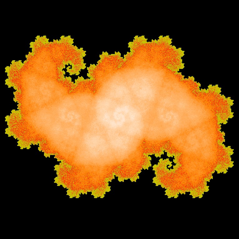
where \({\bf{r}} = \frac{1}{{\sqrt 2 }}\). If H is the unique attractor for this IFS, then
\[H = h_1(H) \cup h_2(H) \cup h_3(H) \cup h_4(H) \]Rotating H by 180° counterclockwise is the same as applying the function g2 from the cyclic group Z2 to the set H. Because g2g2 = g1 (identity) and g2g1 = g2, we get
\[\begin{align} {g_2}(H) &= {g_2}\left( {{h_1}(H) \cup {h_2}(H) \cup {h_3}(H) \cup {h_4}(H)} \right)\\ \\ &= {g_2}{g_1}{f_1}(H) \cup {g_2}{g_2}{f_1}(H) \cup {g_2}{g_1}{f_2}(H) \cup {g_2}{g_2}{f_2}(H)\\ \\ &= {g_2}{f_1}(H) \cup {g_1}{f_1}(H) \cup {g_2}{f_2}(H) \cup {g_1}{f_2}(H)\\ \\ &= h_2(H) \cup h_1(H) \cup h_4(H) \cup h_3(H) = H \end{align}\]This shows that H has 180° rotational symmetry. Also notice that h1(H) = h2(H). That is because h2 does the same scaling to H as h1 but rotates the scaled object 135° clockwise rather than 45° counterclockwise. Because of the 180° rotational symmetry of H, however, the result will be the same in both cases. You can see what happens by clicking on each of the buttons to the left to cover H with the four scaled and rotated copies.
The figure below shows the orbit of the point (0,0) under iteration by the fourth function in the IFS. The orbit spirals into the fixed point of h4. That fixed point is located at (−1,1) since
\[{h_4}\left( {\left[ {\begin{array}{*{20}{c}}{ - 1}\\1\end{array}} \right]} \right) = \left[ {\begin{array}{*{20}{c}}{1/2}&{1/2}\\{ - 1/2}&{1/2}\end{array}} \right]\left[ {\begin{array}{*{20}{c}}{ - 1}\\1\end{array}} \right] + \left[ {\begin{array}{*{20}{c}}{ - 1}\\0\end{array}} \right] = \left[ {\begin{array}{*{20}{c}}0\\1\end{array}} \right] + \left[ {\begin{array}{*{20}{c}}{ - 1}\\0\end{array}} \right] = \left[ {\begin{array}{*{20}{c}}{ - 1}\\1\end{array}} \right]\]
As shown above, the Z2 Heighway dragon has symmetric spirals in the second and the fourth quadrants. This next figure shows a close-up zoom of the spiral in the second quadrant (on a grid of size 1/6 x 1/6).
The white "lakes" inside the red dragon spiral through 45° angles (clockwise), with each lake just touching the one before and the one after as indicated at the dots in the figure. The dot in the upper right where the first lake begins is located at the point (−2/3,1) [Details]. The other dots are the orbit of this point under iteration by the function h4 in the IFS. The first few are (−5/6, 5/6), (−1, 5/6), (−13/12, 11/12), and (−13/12, 1). The orbit converges to the fixed point at (−1,1).
The white lakes in the fourth quadrant exhibit similar behavior with points that are symmetrically opposite from those in the second quadrant.
Z2 Heighway dragon |
Z2 Lévy dragon |
The reason for this is that after composing the transformations in Z2 with the functions in the Heighway IFS and the Lévy IFS, respectively, the new iterated function systems both involve scaling by \(1/\sqrt{2}\) and rotations by 45°, 135°, −45°, and −135°, so they have the same matrices in both systems. The difference is that the translation vectors for the Z2 Lévy dragon are rotated 135° clockwise from those for the Z2 Heighway dragon and scaled by \(1/\sqrt{2}\). This causes the attractor for the Z2 Lévy dragon to be rotated clockwise by 135° and scaled by \(1/\sqrt{2}\) relative to the Z2 Heighway dragon [Proof].
Red: Heighway
Blue: Lévy
|
\({k_1}({\bf{x}}) = \left[ {\begin{array}{*{20}{c}}
{1/2} & { - 1/2} \\
{1/2} & {1/2} \\
\end{array}} \right]{\bf{x}}\) |
scale by r, rotate by 45° |
|
\({k_2}({\bf{x}}) = \left[ {\begin{array}{*{20}{c}}
{-1/2} & { 1/2} \\
{-1/2} & {-1/2} \\
\end{array}} \right]{\bf{x}}\) |
scale by r, rotate by −135° |
|
\({k_3}({\bf{x}}) = \left[ {\begin{array}{*{20}{c}}
{ 1/2} & { 1/2} \\
{-1/2} & { 1/2} \\
\end{array}} \right]{\bf{x}} + \left[ {\begin{array}{*{20}{c}}
1/2 \\
1/2 \\
\end{array}} \right]\) |
scale by r, rotate by −45° |
|
\({k_4}({\bf{x}}) = \left[ {\begin{array}{*{20}{c}}
{ - 1/2} & { - 1/2} \\
{1/2} & { - 1/2} \\
\end{array}} \right]{\bf{x}} + \left[ {\begin{array}{*{20}{c}}
-1/2 \\
-1/2 \\
\end{array}} \right]\) |
scale by r, rotate by 135° |
Note that the matrix for function k3 corresponds to the matrix for function h4, and that the matrix for function k4 corresponds to the matrix for function h3. Also notice that the translation vectors for these functions satisfy the following calculations for a clockwise rotation of 135° and a scaling by \(1/\sqrt{2}\):
\(\dfrac{1}{{\sqrt 2 }}\left[ {\begin{array}{*{20}{c}} {\cos ( - {{135}^ \circ })} & { - \sin ( - {{135}^ \circ })} \\ {\sin ( - {{135}^ \circ })} & {\cos ( - {{135}^ \circ })} \\ \end{array}} \right]\left[ {\begin{array}{*{20}{c}} 1 \\ 0 \\ \end{array}} \right] = \left[ {\begin{array}{*{20}{c}} { - 1/2} & {1/2} \\ { - 1/2} & { - 1/2} \\ \end{array}} \right]\left[ {\begin{array}{*{20}{c}} 1 \\ 0 \\ \end{array}} \right] = \left[ {\begin{array}{*{20}{c}} { - 1/2} \\ { - 1/2} \\ \end{array}} \right]\)and
\(\dfrac{1}{{\sqrt 2 }}\left[ {\begin{array}{*{20}{c}} {\cos ( - {{135}^ \circ })} & { - \sin ( - {{135}^ \circ })} \\ {\sin ( - {{135}^ \circ })} & {\cos ( - {{135}^ \circ })} \\ \end{array}} \right]\left[ {\begin{array}{*{20}{c}} -1 \\ 0 \\ \end{array}} \right] = \left[ {\begin{array}{*{20}{c}} { - 1/2} & {1/2} \\ { - 1/2} & { - 1/2} \\ \end{array}} \right]\left[ {\begin{array}{*{20}{c}} -1 \\ 0 \\ \end{array}} \right] = \left[ {\begin{array}{*{20}{c}} { 1/2} \\ { 1/2} \\ \end{array}} \right]\)More details on symmetric fractals can be found here and in the book by Field and Golubitsky.