Classic Iterated Function Systems

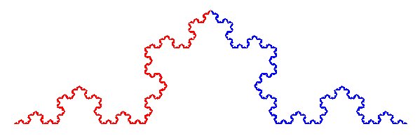
Cesàro's Construction of the Koch Curve

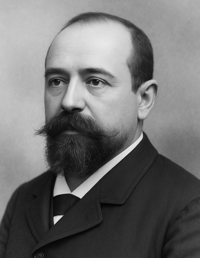
"It is this similarity between the whole and its parts, even infinitesimal ones, which leads us to consider the von Koch curve as a truly spectacular line among all. If it were endowed with life, it would be impossible to annihilate it without eliminating it from the outset, because it would constantly resurface from the depths of its triangles, like life in the Universe!"

E. Cesàro, Atti d. R. Accademia d. Scienze d. Napoli, 2, XII, number 15.

In a 1905 article, Ernesto Cesàro provided an alternative construction of the Koch curve. He starts the construction the same way as Koch. Let \(AB\) be a line segment designated as \(L_0\). Divide \(AB\) into three equal segments \(AD\), \(DE\), and \(EB\) and replace the middle segment by two others \(DC\), \(DE\), forming with \(DE\), to the left of an observer who would move from \(A\) to \(B\), an equilateral triangle. The line \(L_0\) is thus changed to \(L_2 = ADCEB\). Now operating on each segment of \(L_2\) as we did on \(L_0\), we then replace \(L_2\) with another line \(L_4\). Continuing in the same way indefinitely constructs a sequence of polygonal lines \(L_{2n}\) that converges to the Koch curve \(L\).

 

Cesàro notes that the line \(L_{2n+2}\) is always, by construction, to the left of \(L_{2n}\), where by the left and right of any line passing through \(A\) and \(B\), we mean the left and right of an observer who would move on the line, going from \(A\) to \(B\). This means that the polygonal lines \(L_{2n}\) will approach indefinitely the right side of \(L\).

The figure below shows that the vertex C of \(L_2\) lies on the line \(L_1=ACB\) and the other vertices fall to the right of \(L_1\).

The line \(L_4\) is composed of four equal parts constructed on the sides of \(L_2\) in the same manner as \(L_2\) is constructed on \(L_0\), so the line \(L_1\) can be replaced by a line \(L_3\) such that there are new vertices on \(L_4\) that lie on \(L_3\) and the other vertices of \(L_4\) fall to the right of \(L_3\). Moreover, the central parts of triangles ADC and CEB have been removed, which amounts to applying to the right of \(L_1\) the fundamental construction of the Koch curve to \(L_1\).

We can continue this indefinitely to get a second series of polygonal lines \(L_1\), \(L_3\), \(L_5\), etc. that will advance towards the left side of the Koch curve as the series of polygonal lines \(L_0\), \(L_2\), \(L_4\), etc. advance towards the right side of the Koch curve.

The result is that the Koch curve is then the limit of the polygonal lines \(L_0\), \(L_1\), \(L_2\), \(L_3\), \(L_4\), \(L_5\), ... . Moreover, the Koch curve is always included in the region between two consecutive polygonal lines. The region between the lines \(L_n\) and \(L_{n+1}\) consists of \(2^n\) isosceles triangles having their bases on \(L_n\), the other sides on \(L_{n+1}\), and all their vertices on the Koch curve. Here is an example with lines \(L_4\) and \(L_5\).

Click on each of the images above to toggle on and off an approximation of the Koch curve (in green) between the red and black polygonal lines.

These observations led Cesàro to the following alternative construction of the Koch curve. Start with a filled isosceles triangle \(T_0\) with angles 120° and 30° and a base of length 1. The height of this triangle is \(\sqrt{3}/6\) and the lengths of the other two sides is \(1/\sqrt{3}\). It can be divided into three triangles of equal areas: two isosceles triangles that are similar to the initial triangle, and an equilateral triangle with side length 1/3. Remove the equilateral triangle to get the set \(T_1\). Now repeat on the two isosceles triangles in \(T_1\) to get the set \(T_2\), and again on the four isosceles triangles in \(T_2\) to get \(T_3\).

 

 

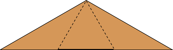
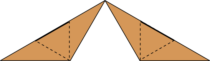
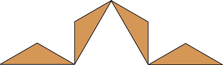
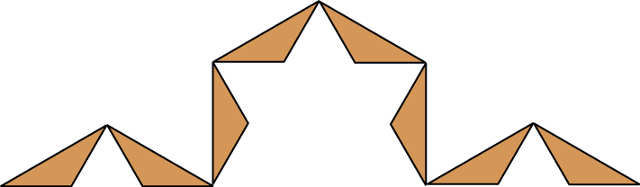
Continue iterating this construction indefinitely to generate a decreasing sequence (\(T_n\)) of connected compact sets that converge to the Koch curve \( \displaystyle K = \bigcap_{n=0}^\infty T_n\), which is therefore also connected and compact [Convergence Details].

Each \(T_n\) consists of \(2^n\) isosceles triangles with base length \((1/\sqrt{3})^n\). The area of \(T_n\) is \((2/3)^n\) of the area of \(T_0\), an area that tends to 0 as \(n\) increases to infinity. As we saw above, the Koch curve is contained entirely inside each \(T_n\) and all the vertices of the triangles in \(T_n\) are points on the Koch curve. Below is an image of \(T_7\).

Cesàro recognized that the Koch curve is "in all its parts self-similar". As he expressed in his paper, "we must think that in each of the triangles of the figure above we embed the entire figure, reduced in a suitable ratio; then that in each of the reduced triangles we insert the entire figure again, and so on, to infinity..." In other words, each of the triangles in \(T_n\) contains its own scaled copy of the Koch curve! This is what Cesàro was referring to in the quote at the top of the page about being impossible to annihilate the Koch curve because "it would constantly resurface from the depths of its triangle."

Cesàro used the self-similarity between the Koch curve and its parts to explain some of the properties found by Koch.

The length of the curve between any two points is infinite. It is sufficient to demonstrate this for the entire curve between the initial point A and final point B. Suppose the length of the curve is the finite value \(l\).

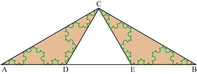
The triangles ACD and BCE in \(T_1\) are similar to triangle ACB (\(T_0\)) and scaled by a factor of \(1/\sqrt{3}\). Therefore the copy of the Koch curve inside triangle ACD is also scaled by a factor of \(1/\sqrt{3}\), as is the copy of the Koch curve inside triangle BCE. Therefore \[l = l/\sqrt{3}+1/\sqrt{3} = 2l/\sqrt{3},\] and this can only be true if \(l = 0\). But that is impossible since \(l > 1\). Therefore the length of the Koch curve cannot be finite.

What is the area \(\sigma\) included between the Koch curve and its chord $AB$?

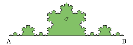
The analogous light green area in triangle ACD and in triangle BCE is the same as the Koch curve area $\sigma$ above scaled by \((1/\sqrt{3})^2 = 1/3\). These areas constitute all of the area of triangle ACB.

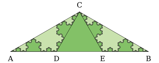
Therefore \[\frac{1}{2}\frac{\sqrt{3}}{6} = \frac{\sigma}{3}+\frac{\sigma}{3}+\sigma = \frac{5}{3}\sigma \quad \Rightarrow \quad \sigma = \frac{\sqrt{3}}{20}.\]

Watch the animation below to see how the two scaled copies of the region between the Koch curve and the base fill in the rest of the area inside the two outer isosceles triangles.

The Koch curve does not have a tangent at any point on the curve. This argument comes from the text by Darst et. al. Suppose P is a point on the Koch curve in the left triangle of \(T_1\), but not equal to vertex C, as shown below. Vertices A, B, C, D, and E are all points on the Koch curve. Let \(\alpha\), \(\beta\), and \(\theta\) be the angles at the three vertices in triangle CEP. Then \(60^\circ \le \alpha \le 90^\circ\) and \(0^\circ \le \beta \le 60^\circ\). Therefore \[60^\circ \le \alpha + \beta \le 150^\circ \quad \Rightarrow \quad 30^\circ \le \theta \le 120^\circ.\] So \(\measuredangle CPE \ge 30^\circ\) which means that the chords PC and PE have slopes that differ by more than \(30^\circ\). If P is a point on the Koch curve in the right triangle of \(T_1\), but again not equal to vertex C, then a similar argument shows that \(\measuredangle CPD \ge 30^\circ\). Finally, if point P is vertex C, then \(\measuredangle APD = 30^\circ\).

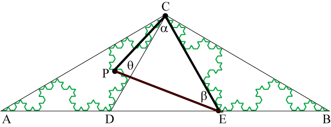
Now suppose \(p\) is any point on the Koch curve. Let \(\delta > 0\). Then \(p\) is a point in one of the isosceles triangle of some set \(T_n\) in the iterative construction of the Koch curve, where the base of the triangle is of length less than \(\delta\) and the triangle is shaped like the figure above. Thus as shown above, there are two points on the Koch curve on one side of \(p\) that are both within a distance \(\delta\) of \(p\) for which the slopes of the chords from \(p\) to the two points differ by more than \(30^\circ\). Since this is true for any \(\delta > 0\), the Koch curve cannot have a tangent at the point \(p\).

Watch a video with more details about why the Koch curve has no tangents using Cesàro's construction.

The first iteration for the Koch curve using the Cesàro construction consists of taking two copies of the initial isosceles triangle \(T_0\), each scaled by \(r = 1/\sqrt{3}\). The red scaled triangle can be obtained by rotating one copy clockwise by 150° and then translated to the point at the top of \(T_0\). The blue scaled triangle can be obtained by rotating the other copy counterclockwise by 150°, then translated to the point (1,0). This yields the following IFS.