Classic Iterated Function Systems

Convergence of the Cesàro Construction

The Hausdorff distance for compact sets

For two non-empty compact subsets \( A, B \subset \mathbb{R}^2 \), the Hausdorff distance is defined as \[ D(A, B) = \max \left\{ \sup_{a \in A} \inf_{b \in B} d(a, b), \sup_{b \in B} \inf_{a \in A} d(b, a) \right\} \] where \(d(a,b)\) is the usual Euclidean distance between the points \(a\) and \(b\). Here \(\displaystyle \inf_{b \in B} d(a, b)\) is the shortest distance of \(a\) to all of the points in \(B\). Now do the same in the other direction and then take the maximum of both to get the Hausdorff distance of set \(A\) from set \(B\). This can be summarized as the maximum of the distances from any point in $A$ to the nearest point in $B$, and the distances from any point in $B$ to the nearest point in $A$. This is a metric on the space of all non-empty compact sets in the plane, so it satisfies all the usual properties of a distance function. It makes the space of non-empty compact subsets a complete metric space.

The distance between sets in the Cesàro construction and the Koch construction

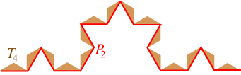
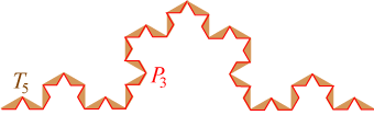
The image below shows the first five iterations in the Cesàro construction in brown. Also illustrated is how the bottom boundary of each iteration is one of the polygonal lines in the Koch construction. The column on the left shows the relationship between the polygonal line \(P_n\) and the corresponding Cesàro isosceles triangles in \(T_{2n}\), while the column on the right shows the corresponding relationship between the polygonal line \(P_n\) and the Cesàro isosceles triangles in \(T_{2n-1}\). We can take \(P_0\) to be of unit length.

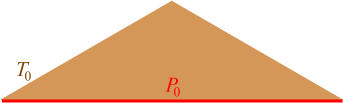
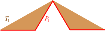
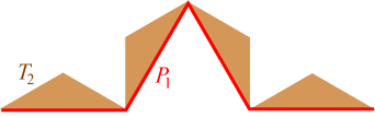
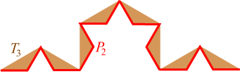
We first find the distance between \(P_n\) and \(T_{2n}\) for the situation in the left column. In each case, the set \(T_{2n}\) consists of isosceles triangles where the base of each triangle is a line segment in \(P_n\) and the other two sides are in \(T_{2n}\). Each of the isosceles triangles in \(T_{2n}\) has the shape shown below.

Since \(P_n\) is a subset of \(T_{2n}\), the distance from each point in \(P_n\) to the set \(T_{2n}\) is 0. Therefore \(\displaystyle \sup_{y \in P_n} \inf_{x \in T_{2n}} d(y,x)=0.\) The drawing shows that the top of the isosceles triangle is the point in \(T_{2n}\) that is farthest from \(P_n\). This distance is the height of an isosceles triangle with a base in \(P_n\) of length \((1/3)^n\). The height is therefore \[ \frac{1}{2}\left(\frac{1}{3}\right)^n\cdot\tan(30^\circ)=\frac{1}{2}\left(\frac{1}{3}\right)^n\cdot\frac{1}{\sqrt{3}}.\] Hence \[D(P_n,T_{2n})=\max\left\{0,\frac{1}{2\sqrt{3}}\left(\frac{1}{3}\right)^n\right\}=\frac{1}{2\sqrt{3}}\left(\frac{1}{3}\right)^n.\]

Next we find the distance between \(P_n\) and \(T_{2n-1}\) for the situation in the right column. The main difference is that the set \(T_{2n-1}\) consists of isosceles triangles where the base of each triangle is a line segment in \(T_{2n-1}\) and the other two sides are in \(P_n\). The isosceles triangles in \(T_{2n-1}\) have the shape shown below.

Now the middle of the base of the isosceles triangle is the point in \(T_{2n-1}\) that is farthest from \(P_n\). This distance is the height of an isosceles triangle with a base in \(T_{2n-1}\) of length \((1/\sqrt{3})^{2n-1}\). The height is therefore \[ \frac{1}{2}\left(\frac{1}{\sqrt{3}}\right)^{2n-1}\cdot\tan(30^\circ)=\frac{1}{2}\left(\frac{1}{3}\right)^n\sqrt{3}\cdot\frac{1}{\sqrt{3}}=\frac{1}{2}\left(\frac{1}{3}\right)^n.\] Hence \[D(P_n,T_{2n-1})=\max\left\{0,\frac{1}{2}\left(\frac{1}{3}\right)^n\right\}=\frac{1}{2}\left(\frac{1}{3}\right)^n.\]

The sequence (\(T_n\)) in the Cesàro construction converges to the Koch curve

We know that the polygonal lines in the Koch construction converge to the Koch curve \(K\). [Proof] This means that \(\displaystyle \lim_{n\rightarrow \infty}D(K,P_n) = 0\). But we also have \[ \lim_{n\rightarrow \infty}D(P_n,T_{2n}) = \lim_{n\rightarrow \infty}\frac{1}{2\sqrt{3}}\left(\frac{1}{3}\right)^n = 0.\] Since \(D(K,T_{2n})\le D(K,P_n)+D(P_n,T_{2n})\) by the triangle inequality for the Hausdorff metric, we can conclude that \(\displaystyle \lim_{n\rightarrow \infty}D(K,T_{2n}) = 0\). A similar argument shows that \(\displaystyle \lim_{n\rightarrow \infty}D(K,T_{2n-1}) = 0\).

So the sequence (\(T_{2n}\)) converges to the Koch curve and the sequence (\(T_{2n-1}\)) also converges to the Koch curve. Therefore the entire sequence (\(T_n\)) from the Cesàro construction converges to the Koch curve.

Note: Convergence via Banach Fixed Point Theorem

Hutchinson's Theorem can also be used to show the convergence of the Cesàro construction. The following iterated function system consists of two contractive maps.

If the Hutchinson operator \(G\) is given by \(G(A) = g_1(A) \cup g_2(A)\) for a non-empty compact set \(A\) in the plane, then \(F\) is a contractive map by Hutchinson's Theorem. Since

and \(F\) is a contraction on a complete metric space, the Banach Fixed Point Theorem guarantees that

1. there exists a unique fixed point \(A^*\) such that \(\displaystyle A^* = G(A^*) = \bigcup_{n=1}^2 g_n(A^*)\);
2. the sequence of sets \(T_n = F(T_{n-1})\) converges to \(A^*\) in the Hausdorff metric.

So the Cesàro construction converges to the IFS fixed point (attractor). We want to show that this attractor is the Koch curve.

Recall that the IFS for the Koch curve is given by four functions \(\{f_1,f_2,f_3,f_4\}\):

The Koch curve is the unique fixed point for the Hutchinson operator \(F(A) = f_1(A) \cup f_2(A) \cup f_3(A) \cup f_3(A)\). The important observation is that \[ g_1 \circ g_1 = f_2 \\ g_1 \circ g_2 = f_1 \\ g_2 \circ g_1 = f_4 \\ g_2 \circ g_2 = f_3 \] This makes sense because, for example, \(g_1 \circ g_1\) means to scale twice by \(1/\sqrt{3}\), so by \(1/3\), and to rotate twice by −150°, so by −300°, or equivalently by 60°. This is what \(f_2\) does. The other three compositions have similar interpretations. So this in turn implies that \(G(G(A)) = F(A)\) for all compact sets A [Calculations (pdf)]. In particular, \[F(A^*) = G(G(A^*) = G(A^*) = A^*.\] But this means that \(A^*\) is the fixed point for the Koch IFS, and thus \(A^*\) must be the Koch curve.